Building a SetFit Dataset: The Data

This is Part 3 of my SetFit series. In Part 1, I explained what SetFit is and why it’s useful. In Part 2, I covered taxonomy design. Now let’s get our hands dirty with the actual data.

From Taxonomy to Training Data

At this point, you have a taxonomy. You know what your categories are and why they exist. But you still don’t have a dataset. And SetFit needs labeled examples to train on.

The gap between “I have a taxonomy” and “I have a training dataset” is wider than it looks. You need to:

1. Extract candidate headlines from your database
2. Pre-label them (because labeling from scratch is slow)
3. Review and correct the labels manually
4. Publish the final dataset somewhere versioned

Each step has trade-offs. None of them is perfect. Let me walk you through what I actually did.

Sampling Headlines with SQL

I have about 500,000 headlines in my PostgreSQL database, collected from ~150 French-language news sources. I don’t need all of them — I need a representative subset that covers my 12 categories well.

There are three sampling strategies I use, depending on the situation.

A Quick Note on CTEs

If you’re not familiar with SQL CTEs (Common Table Expressions), they’re the WITH ... AS blocks you’ll see throughout this article. Think of them as temporary named queries — like variables for SQL results. They make complex queries readable by breaking them into logical steps instead of nesting subqueries inside subqueries.

-- Without CTE: hard to read
SELECT * FROM (
    SELECT *, ROW_NUMBER() OVER (...) AS rn
    FROM (SELECT * FROM headlines WHERE ...) h
) ranked WHERE rn <= 50;

-- With CTE: each step has a name
WITH filtered AS (
    SELECT * FROM headlines WHERE ...
),
ranked AS (
    SELECT *, ROW_NUMBER() OVER (...) AS rn FROM filtered
)
SELECT * FROM ranked WHERE rn <= 50;

You’ll also see ROW_NUMBER() OVER (PARTITION BY ... ORDER BY ...). This is a window function — it assigns a number to each row within a group (partition). Combined with a filter like WHERE rn <= 50, it lets you pick the top N rows per group. Very useful for balanced sampling.

Strategy 1: Sample by Existing Classification

If you already have a working pipeline with labels (even imperfect ones), you can sample directly from it. This is useful when you’re improving an existing model, not building one from scratch.

WITH category_sample AS (
    SELECT
        h.id,
        COALESCE(
            (h.title_translation->>'fr')::text,
            h.title
        ) AS title,
        h.source_slug,
        h.source_lang,
        s.country,
        h.setfit_category_id,
        sc.name AS category_name
    FROM (
        SELECT h.*,
            ROW_NUMBER() OVER (
                PARTITION BY h.setfit_category_id
                ORDER BY RANDOM()
            ) AS rn
        FROM headlines h
        INNER JOIN sources s ON h.source_slug = s.slug
        WHERE h.setfit_category_id IS NOT NULL
          AND h.published_at < '2025-12-15'
          AND s.is_active = true
          AND (s.political_side IS NULL
               OR s.political_side != 'far-right')
    ) h
    INNER JOIN sources s ON h.source_slug = s.slug
    INNER JOIN setfit_categories sc
        ON h.setfit_category_id = sc.id
    WHERE h.rn <= 50
)
SELECT * FROM category_sample ORDER BY RANDOM();

What this does:

• PARTITION BY h.setfit_category_id: Groups headlines by their current category
• ORDER BY RANDOM(): Shuffles within each group so we get different headlines each time
• WHERE h.rn <= 50: Takes at most 50 headlines per category
• COALESCE(title_translation->>'fr', title): Uses the French translation if available, otherwise the original title (some sources publish in other languages)

The result is a balanced dataset: 50 headlines per category, drawn randomly from the existing classifications. The cutoff date (published_at < '2025-12-15') ensures I’m not training on data that the model has already seen in production.

I also add a second CTE for recently added sources, to make sure new sources are represented:

recent_source_sample AS (
    SELECT ...
    FROM (
        SELECT h.*,
            ROW_NUMBER() OVER (
                PARTITION BY h.source_slug
                ORDER BY RANDOM()
            ) AS rn
        FROM headlines h
        INNER JOIN sources s ON h.source_slug = s.slug
        WHERE h.setfit_category_id IS NOT NULL
          AND s.created_at > '2025-09-07'  -- recently added
          ...
    ) h
    WHERE h.rn <= 10  -- 10 per source
)

Then I combine both with UNION (which also deduplicates) and shuffle:

combined AS (
    SELECT * FROM category_sample
    UNION
    SELECT * FROM recent_source_sample
)
SELECT * FROM combined ORDER BY RANDOM();

When to use this: You have an existing classifier and want to build a better dataset for the next version. The current labels give you a starting point — you’ll correct errors during review.

Strategy 2: Targeted Sampling for Specific Categories

Sometimes you need more data for categories that are under-represented or newly added. For this, I use keyword-based filtering to find likely candidates.

For example, to find headlines about Swiss politics:

WITH swiss_headlines AS (
    SELECT
        h.id,
        CASE
            WHEN h.source_lang = 'fr' THEN h.title
            ELSE (h.title_translation->>'fr')::text
        END as title,
        h.source_slug,
        s.country,
        'Politique Suisse' as target_category
    FROM headlines h
    JOIN sources s ON h.source_slug = s.slug
    WHERE s.country = 'CH'
      AND s.is_active = true
      AND s.political_side != 'far-right'
      AND h.published_at >= CURRENT_DATE - INTERVAL '30 days'
      AND h.title IS NOT NULL
      AND LENGTH(h.title) > 20
    ORDER BY RANDOM()
    LIMIT 200
)
SELECT * FROM swiss_headlines;

For more specific categories, I use keyword patterns. Here’s how I find developer-focused technical content:

WITH tech_headlines AS (
    SELECT ...
    FROM headlines h
    JOIN sources s ON h.source_slug = s.slug
    WHERE s.category IN ('tech', 'science')
      AND (
        -- Programming keywords
        h.title ILIKE '%developer%' OR
        h.title ILIKE '%API%' OR
        h.title ILIKE '%Python%' OR
        h.title ILIKE '%JavaScript%' OR
        h.title ILIKE '%open source%' OR
        h.title ILIKE '%GitHub%' OR
        -- ML/AI keywords
        h.title ILIKE '%machine learning%' OR
        h.title ILIKE '%LLM%' OR
        h.title ILIKE '%transformer%' OR
        -- DevOps keywords
        h.title ILIKE '%Kubernetes%' OR
        h.title ILIKE '%Docker%' OR
        h.title ILIKE '%CI/CD%'
      )
    ORDER BY RANDOM()
    LIMIT 250
)
SELECT * FROM tech_headlines;

Notice the LIMIT 250 when my target is 100 samples. I use a 2.5x safety margin — I sample more than I need because not every headline will match the category after human review. Some will be false positives from the keyword filter, and some will be duplicates or low-quality headlines I’ll want to remove.

When to use this: You’re adding a new category or the current dataset is weak for a specific class. Keyword filtering gives you a focused pool to review.

Strategy 3: Proportional Sampling by Source Distribution

This is the most interesting strategy. The idea: sample headlines proportionally to how they’re distributed across sources in real life. If Le Monde represents 8% of your headlines, you want roughly 8% of your sample to come from Le Monde.

Why does this matter? If you sample randomly without thinking about sources, you’ll likely over-represent high-volume sources and under-represent small ones. Your model will learn the vocabulary of Le Figaro but struggle with the writing style of a Swiss newspaper.

WITH source_stats AS (
    SELECT
        s.slug AS source_slug,
        s.name AS source_name,
        s.country,
        COUNT(h.id) AS headlines_count,
        GREATEST(1,
            ROUND(
                COUNT(h.id)::NUMERIC
                / SUM(COUNT(h.id)) OVER()
                * 2000
            )
        ) AS sample_size
    FROM headlines h
    JOIN sources s ON h.source_slug = s.slug
    WHERE s.is_active = true
      AND s.exclude_from_clustering = false
      AND s.political_side != 'far-right'
      AND h.published_at >= CURRENT_DATE - INTERVAL '30 days'
      AND h.title IS NOT NULL
      AND LENGTH(h.title) > 20
    GROUP BY s.slug, s.name, s.country
),
sampled_headlines AS (
    SELECT
        h.id,
        CASE
            WHEN h.source_lang = 'fr' THEN h.title
            ELSE (h.title_translation->>'fr')::text
        END as title,
        h.source_slug,
        ROW_NUMBER() OVER (
            PARTITION BY h.source_slug
            ORDER BY RANDOM()
        ) AS rn,
        ss.sample_size
    FROM headlines h
    JOIN source_stats ss ON h.source_slug = ss.source_slug
    WHERE h.published_at >= CURRENT_DATE - INTERVAL '30 days'
)
SELECT id, title, source_slug
FROM sampled_headlines
WHERE rn <= sample_size;

The key line is:

GREATEST(1, ROUND(COUNT(h.id)::NUMERIC / SUM(COUNT(h.id)) OVER() * 2000)) AS sample_size

Breaking it down:

• COUNT(h.id): how many headlines this source has
• SUM(COUNT(h.id)) OVER(): total headlines across all sources (a window function with no partition — it sums everything)
• Divide one by the other: the source’s proportion (e.g., 0.08 for 8%)
• Multiply by 2000: the target total sample size
• GREATEST(1, ...): ensure every source gets at least 1 headline, even small ones

Then in the second CTE, ROW_NUMBER() OVER (PARTITION BY h.source_slug ORDER BY RANDOM()) shuffles headlines within each source, and WHERE rn <= sample_size keeps only the calculated number.

When to use this: You want a representative dataset that reflects the real distribution of your data. Good for building a general-purpose classifier, less good for under-represented categories (use Strategy 2 for those).

No Strategy Is Perfect

In practice, I go back and forth between all three. Strategy 1 gives me a quick balanced dataset when I already have labels. Strategy 2 fills gaps for specific categories. Strategy 3 gives me a realistic distribution for general evaluation.

The dataset is built incrementally: sample, label, train, evaluate, find the weak spots, sample more targeted data, re-label, re-train. It’s not a linear process.

Using an LLM to Pre-Classify Headlines

Labeling hundreds of headlines from scratch is slow. But if someone gives you a pre-filled spreadsheet where 70-80% of the labels are already correct, you’re just reviewing and correcting. That’s much faster.

That “someone” is a cheap LLM.

The Prompt

I use a structured YAML prompt that feeds headlines to Claude Haiku 4.5. Here’s the structure (simplified — the full prompt has 12 categories):

name: "v2-202601-classifier"
version: "1.0.0"

instructions: |
  You are an expert in classifying French and international
  news headlines.
  Classify each headline into ONE category among the 12 listed.

prompt: |
  <task>
  Classify the following headlines according to the taxonomy.
  For each headline, return the id, setfit_category_id, and category.
  </task>

  <taxonomy>
  <category id="1" name="Politique FR, EU, Quebec">
    <description>
      All political news from the Western francophone world
      and Europe.
    </description>
    <includes>
      - French, Belgian, Swiss, Quebec political parties
      - Local, regional, national elections in Europe
      - Laws and reforms voted in France/Europe
    </includes>
    <excludes>
      - If an actor is OUTSIDE Europe (USA, Russia, China)
        -> category 2
      - Social debates without direct political dimension
        -> category 4
    </excludes>
    <examples>
      - "Macron announces pension reform" -> 1
      - "EU Parliament votes AI directive" -> 1
    </examples>
  </category>

  <category id="3" name="Economie & Marches & Business Tech">
    ...
    <differentiation>
      IMPORTANT - Business Tech vs Code & Infrastructure:
      - "OpenAI raises 6 billion" -> 3 (investment)
      - "How to use the OpenAI API" -> 13 (tutorial)
      - "Samsung Galaxy test" -> 10 (product review)
      - "Apple acquires an AI startup" -> 3 (acquisition)
    </differentiation>
  </category>
  </taxonomy>

  <headlines>
  {{ headlines_json }}
  </headlines>

config:
  model: "claude-haiku-4-5"
  temperature: 0.1
  max_tokens: 4000

Why This Structure Works

A few design choices worth explaining:

XML tags in the prompt. I use <includes>, <excludes>, <examples>, and <differentiation> sections for each category. This forces me to think about boundaries, not just definitions. What does this category include? What does it explicitly exclude? Where does it overlap with another category, and how do I resolve the ambiguity?

The <differentiation> block is especially useful. Categories 3 (Business Tech) and 13 (Code & Infrastructure) overlap a lot in the tech space. Concrete examples with arrows make the distinction clear:

• “OpenAI raises 6 billion” → 3 (it’s a funding round, business news)
• “How to use the OpenAI API” → 13 (it’s a developer tutorial)
• “Samsung Galaxy test” → 10 (it’s a product review for consumers)

Why Claude Haiku 4.5? Two reasons:

1. Cost: Haiku is cheap. At ~$0.25 per million input tokens, classifying 2,000 headlines costs about$0.50. Even if I run it three times for consistency checks, it’s under $2.
2. Speed: Haiku is fast. 2,000 headlines in a few minutes.

I don’t need Sonnet or Opus for this. The LLM is not making the final decision — it’s giving me a head start. I expect 20-30% of its labels to be wrong, and I’ll fix those during review.

Why temperature 0.1? I want consistency, not creativity. If I run the same batch twice, I want roughly the same labels. Temperature 0.1 keeps the model deterministic without being fully greedy (temperature 0 can sometimes get stuck in loops).

This Is Not Your Final Label

I want to stress this: the LLM pre-classification is not the ground truth. It’s a time-saver. The workflow is:

1. Sample headlines with SQL → export to CSV
2. Run the LLM classifier → add a llm_category column to the CSV
3. Open the CSV in the review tool → correct labels manually
4. Export the corrected CSV → that’s your training data

The LLM turns a 4-hour labeling session into a 1.5-hour review session. That’s the value.

A Custom Streamlit Tool for Human Review

Why Not Label Studio?

Label Studio is the go-to tool for data labeling. It’s powerful, handles images, audio, text, and complex annotation tasks. But for classifying headlines into categories — picking one label from a dropdown for each row — it’s too much.

Label Studio requires a server, a database, project setup, import/export configuration, and a learning curve. I needed something I could start in 30 seconds and close when I’m done.

Streamlit is perfect for this: a Python script that becomes a web app. No frontend code, no deployment, no database. Run streamlit run app.py, and you have a review tool.

The Review Interface

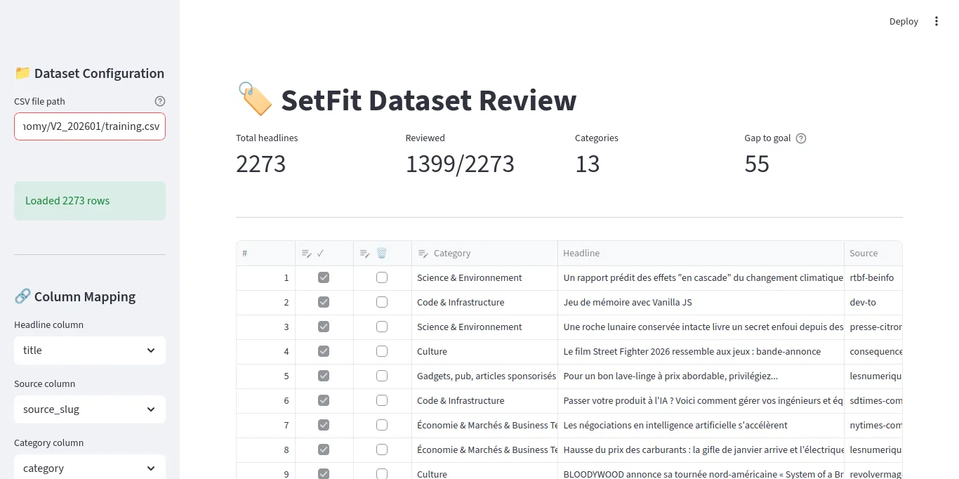
The core of the tool is Streamlit’s data_editor — a spreadsheet-like widget with typed columns:

edited_df = st.data_editor(
    work_df,
    column_config={
        "#": st.column_config.NumberColumn(
            "#", disabled=True, width="small"
        ),
        "reviewed": st.column_config.CheckboxColumn(
            "✓", help="Mark as reviewed", width="small"
        ),
        "delete": st.column_config.CheckboxColumn(
            "🗑️", help="Mark for deletion", width="small"
        ),
        "category": st.column_config.SelectboxColumn(
            "Category",
            options=categories,
            required=True,
            width="medium"
        ),
        "headline": st.column_config.TextColumn(
            "Headline", disabled=True, width="large"
        ),
        "source": st.column_config.TextColumn(
            "Source", disabled=True, width="small"
        ),
    },
    hide_index=True,
    use_container_width=True,
)

Six columns: row number, reviewed checkbox, delete checkbox, category dropdown, headline text, and source name. The headline and source columns are read-only (disabled=True) — you can only change the checkbox and category.

Key Features

Browser persistence with localStorage. I use streamlit-local-storage to save the CSV path, categories file path, and target goal in the browser. When I close the tab and come back, everything is where I left it.

from streamlit_local_storage import LocalStorage
localS = LocalStorage()

# Restore CSV path from last session
saved_csv_path = localS.getItem("csv_file_path") or ""
csv_path = st.text_input("CSV file path", value=saved_csv_path)

# Save if changed
if csv_path and csv_path != saved_csv_path:
    localS.setItem("csv_file_path", csv_path, key="set_csv_path")

Automatic backup. The first time you load a CSV, it creates a .bak copy. If you mess things up, you can restore from the backup.

backup_path = Path(f"{csv_path}.bak")
if not backup_path.exists():
    shutil.copy(csv_path, backup_path)

Category distribution chart. An expandable section shows how many reviewed headlines exist per category. This helps me see which categories need more work.

Gap to goal metric. I set a target (default: 55 reviewed headlines per category) and the UI shows which category is furthest from that goal. This guides my review — I focus on categories that need more labels.

Saving Your Work

The Sync button saves edits back to the CSV, removes deleted rows, and converts booleans to t/f strings:

if st.button("🔄 Sync", type="primary"):
    to_delete_mask = edited_df["delete"]
    keep_mask = ~to_delete_mask
    kept_indices = edited_df[keep_mask].index.tolist()

    df_filtered = df.iloc[kept_indices].copy()
    df_filtered[category_col] = edited_df.loc[keep_mask, "category"].values
    df_filtered["reviewed"] = edited_df.loc[keep_mask, "reviewed"].apply(
        lambda x: "t" if x else "f"
    )

    df_filtered.to_csv(csv_path, index=False)

This is important: the tool edits the CSV in place. No database, no export step. You work directly on the file that will become your training data.

Notes on Manual Classification

The labeling itself is the boring part. But there are a few things I learned that made it less painful.

Column Order Matters

This sounds trivial, but it’s not. The order of columns in the spreadsheet directly affects your speed.

My layout: # | ✓ | 🗑️ | category | headline | source

The checkbox and dropdown are next to each other, on the left. The headline text is right after them. This means I read the headline, then move my mouse slightly left to check “reviewed” and pick a category. Minimal movement.

If I put the headline first and the category last, I’d be scrolling or moving my mouse across the entire screen for every single row. Over 500 rows, that adds up.

Keep Notes on Borderline Decisions

Some headlines could reasonably go in two categories. “Macron meets Zelensky to discuss military aid” — is that French politics (category 1) or geopolitics (category 2)?

My rule: Russia/Ukraine = outside Europe = geopolitics (category 2). I wrote this rule in the LLM prompt’s <key_rule> tag, and I follow the same rule during manual labeling.

The point is: when you make a borderline call, write down your reasoning. Keep a simple text file or a note in your prompt file. You’ll need it when you review the model’s mistakes later and wonder “why did I label this one differently?”

Consistency matters more than being “right.” If you always classify Ukraine headlines as geopolitics, the model learns that pattern. If you sometimes pick politics and sometimes geopolitics, the model learns noise.

Don’t Aim for Perfection

You don’t need to review every single headline. SetFit works with small datasets — 50-80 well-labeled examples per category is enough for a first pass. If a category has 55 good labels, move on to the next one. You can always come back and add more in the next iteration.

Publishing the Dataset to Hugging Face

Once your CSV is reviewed and clean, you have a training dataset. But a CSV on your laptop is fragile — one bad git clean and it’s gone. And when you want to train on a remote GPU (I use RunPod for this), you need a way to get the data there without manual file transfers.

The Hugging Face Hub solves both problems: it versions your dataset and makes it loadable in one line from any machine.

The Upload Script

I use Hugging Face’s datasets library to push a clean dataset with train/test splits:

import os
import pandas as pd
from datasets import Dataset, DatasetDict, Features, Value
from huggingface_hub import login
from dotenv import load_dotenv

load_dotenv()

HF_TOKEN = os.getenv("HF_TOKEN")
HF_OWNER = os.getenv("HF_OWNER")
HF_REPO = os.getenv("HF_REPO")

login(token=HF_TOKEN)

def create_dataset(csv_file, split_name):
    df = pd.read_csv(csv_file)
    df = df.dropna(subset=['category'])
    df = df.reset_index(drop=True)

    features = Features({
        'headline': Value('string'),
        'category': Value('string'),
        'source': Value('string')
    })

    return Dataset.from_pandas(df, features=features)

train_dataset = create_dataset("data/train.csv", "train")
test_dataset = create_dataset("data/test.csv", "test")

dataset_dict = DatasetDict({
    'train': train_dataset,
    'test': test_dataset
})

repo_id = f"{HF_OWNER}/{HF_REPO}"
dataset_dict.push_to_hub(repo_id, private=False)

A few things to note:

• Features define the schema. By declaring types explicitly, you avoid Hugging Face guessing wrong (it sometimes infers integers for string columns that happen to look like numbers).
• push_to_hub handles everything: creates the repo if it doesn’t exist, uploads the data in Parquet format, generates a dataset card.
• Train/test split. I split the reviewed CSV before uploading. A typical split: 80% train, 20% test. Stratified by category so each split has the same category distribution.

Why This Matters

Once the dataset is on the Hub, loading it from a training notebook is one line:

from datasets import load_dataset

dataset = load_dataset("afk-live/setfit-headlines-v2")
train_dataset = dataset["train"]
test_dataset = dataset["test"]

This works from anywhere — your laptop, a RunPod instance, Google Colab. No file paths, no scp, no volume mounts. The data is versioned and reproducible.

It also acts as an archive. When I retrain with a new taxonomy or more data, I push a new dataset version. The naming convention is simple: setfit-headlines-v2, setfit-headlines-v3, etc. If a new version produces a worse model, I can point the training script at the previous dataset and reproduce the old results.

The Dataset Card

Just like models have model cards, datasets have dataset cards. Hugging Face generates a basic one from the Features definition, but I recommend adding your taxonomy to it. When you come back 3 months later wondering “what were the categories in v2?”, the dataset card should have the answer.

The Full Workflow

Putting it all together:

1. SQL sampling  ──→  raw_headlines.csv
2. LLM pre-label ──→  preclassified_headlines.csv (+ llm_category column)
3. Streamlit      ──→  reviewed_headlines.csv (corrected + reviewed flags)
4. Train/test split ─→ train.csv + test.csv
5. Hugging Face   ──→  versioned dataset on the Hub

Each step feeds the next. The CSV is the common format between all steps — no special tools, no proprietary formats. You can open it in any spreadsheet app if Streamlit is not available.

And because the final dataset is on Hugging Face, loading it into a training notebook is trivial — which is exactly what we’ll do next.

What’s Next

In Part 4, I’ll cover the actual training: setting up a RunPod instance, SetFit training arguments, evaluation metrics, and the train-evaluate-iterate loop that turns a dataset into a production classifier.

---

This article is part of my journey learning ML as a senior engineer without a data science background. I’m documenting what I learn, including the mistakes, because the polished tutorials rarely show the messy reality of building ML systems.