The z-score, an old friend you keep meeting in ML

I started exploring ML a couple of years ago coming from a “computer science old school” background — twenty years of building systems, very little hands-on with statistics. As I dig into NLP and trend detection, I keep bumping into one indicator that I had vaguely seen in high school and forgotten about: the z-score.

It is one of those tools that feels almost too simple to be useful, and yet I have now used it in two completely different parts of my project AFK, a news aggregation platform that builds editorial trends out of journalistic work. I would like to share both usages here, because they show how the same elementary idea — how many standard deviations away from the mean am I? — can be applied at very different scales, with very different goals.

This is part of an ongoing series where I write down what I learn as I go. As before, I’ll share the formal definition, the intuition, and the actual code that runs in production.

The z-score, back to basics

Given a value $x$ , a mean $\mu$ and a standard deviation $\sigma$ , the z-score of $x$ is:

z = \frac{x - \mu}{\sigma}

That is it. The numerator measures how far $x$ is from the average, the denominator expresses that distance in units of standard deviation. The result is dimensionless: a z-score of 2 means “twice the typical spread above average”, whether the underlying quantity is mentions per day, word frequencies, or stock returns.

If the underlying distribution is roughly normal (the famous bell curve), the 68-95-99.7 rule gives an immediate intuition for the thresholds:

about 68% of values fall within $\pm 1\sigma$
about 95% within $\pm 2\sigma$
about 99.7% within $\pm 3\sigma$

The 68-95-99.7 rule on a standard normal distribution

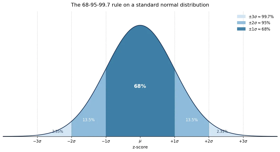
So a z-score above 2 is “uncommon” (one event in twenty), above 3 is “rare” (three events in a thousand). The thresholds I’ll show below — 2.5 and 3.5 — sit between those landmarks and are calibrated empirically rather than from a theoretical p-value.

A natural reflex is to ask: but my data is not normal! True. The 68-95-99.7 rule strictly speaking only applies to a Gaussian, and entity counts in news data, or word frequencies in a corpus, are very far from Gaussian (they tend to be heavily right-skewed, often closer to a power law). The z-score still works as an ordering tool — it ranks deviations consistently, even when the absolute probability interpretation doesn’t hold. In practice, this is what we use it for: finding the entities or terms whose deviation stands out relative to their peers, rather than computing a strict statistical significance.

With that out of the way, let’s look at the two usages.

Usage 1 — Temporal anomaly detection on entity counts

In AFK, every morning I extract named entities (people, organisations, locations) from hundreds of fresh news headlines. Over time, the database accumulates a daily count per entity: how many times “Macron” was mentioned on April 12, on April 13, on April 14, and so on. The question I want to answer at the end of each batch is:

Which entities are unusually loud today, given their own recent history?

This is anomaly detection on a time series, and the z-score is a very natural fit. For each entity, I take a sliding window of the last 14 days, compute the mean and standard deviation of the daily mention count, and z-score today’s value against those baseline statistics:

# gen-output/enr/analytics/anomaly_detector.py

Z_SCORE_THRESHOLD = 2.5  # Breakout detection threshold
CRITICAL_Z_SCORE = 3.5   # Critical anomaly threshold


def calculate_z_score(
    current_value: float,
    mean: float,
    std: float
) -> float:
    if std is None or std == 0:
        return 0.0
    return (current_value - mean) / std


def is_anomaly(z_score: float, threshold: float = Z_SCORE_THRESHOLD) -> bool:
    return abs(z_score) >= threshold

The baseline statistics come straight from PostgreSQL with a one-shot aggregate over the entity’s daily counts:

SELECT
    AVG(daily_total) AS mean,
    STDDEV(daily_total) AS std,
    COUNT(*) AS sample_size
FROM (
    SELECT SUM(total_count) AS daily_total
    FROM entity_daily_counts
    WHERE entity_id = %s
      AND count_date < %s
      AND count_date >= %s - INTERVAL '%s days'
    GROUP BY count_date
) daily_totals

A few practical details that turn out to matter quite a lot:

Minimum sample size. The function refuses to compute a z-score if it has fewer than 3 days of history. With one or two data points the standard deviation is meaningless or zero; either case produces wild scores.
Guard against std == 0. If an entity was mentioned exactly the same number of times every day, $\sigma = 0$ and the z-score formula divides by zero. I return 0.0 in that case rather than raising — the entity is, by definition, not anomalous.
Two thresholds, not one. 2.5 flags a “breakout” (worth surfacing), 3.5 flags a “critical” anomaly (worth highlighting). Splitting the alert into two tiers gives editorial control downstream.
Absolute value. The detector flags both spikes and collapses (abs(z_score) >= threshold). An entity that suddenly stops being mentioned can be just as informative as one that explodes — think of a public figure disappearing from headlines after a scandal subsides.

The window length (14 days) is itself a tuning knob. A short window is reactive but noisy: every story that runs hot for a week becomes its own baseline and stops looking anomalous on day three. A long window is stable but slow: a politician who has been ramping up for two months may never trigger. 14 days is a pragmatic compromise for daily news; for slower media or social-media bursts, you would pick differently.

Going further — z-score for time series in general

This pattern — rolling mean, rolling standard deviation, threshold on the z-score — is one of the simplest and most common forms of unsupervised anomaly detection on time series. It shows up everywhere: server-load monitoring, fraud detection, IoT sensor outliers, financial market microstructure. It is often the first baseline you should try before reaching for anything fancier (Isolation Forest, LSTM autoencoders, Prophet residuals…), because:

it has essentially no hyperparameters beyond the window length and the threshold;
it is interpretable — you can show a non-technical user the chart, the baseline band, the spike;
it scales trivially: per-entity statistics fit in a single SQL aggregate.

Common refinements include robust statistics (median and median-absolute-deviation instead of mean and standard deviation, to resist the influence of past spikes), EWMA (exponentially weighted moving averages, which give more weight to recent days), and seasonality removal (subtract a weekly or daily cycle before z-scoring). All of them keep the z-score at the heart of the decision; they just feed it cleaner inputs.

Usage 2 — Which words best discriminate two corpora?

The second usage is further from a textbook z-score, and it took me longer to recognise the same indicator hiding inside a more elaborate formula. The problem is one any text analyst eventually faces, and we’ll arrive at the z-score by gradually fixing the flaws of a naive approach. Bear with me — the destination is worth the detour.

In AFK, one of the editorial pipelines analyses political speeches and op-eds against the four-attractor geometry that Bruno Latour proposes in Où atterrir? (2017): Terrestre, Global, Hors-Sol, Local. Each pole is described in code by a list of “seed phrases” — short snippets that capture the rhetoric of that pole — and an incoming text is projected against those seeds via embedding cosine similarity.

The hard part is bootstrapping the seeds. Rather than pick them by intuition, I built a labelled corpus of texts whose pole is editorially known, and asked a more concrete question:

Among all the words that appear in this corpus, which ones are over-represented in pole P relative to the three other poles?

This is the classic problem of comparing the vocabulary of two corpora — finding the words that “belong” to one side rather than the other. The natural temptation is to compare raw frequencies: “the word territoire appears 45 times in Terrestre texts and 12 times in the rest, therefore it is Terrestre-discriminative.” But this is unreliable for two well-known reasons:

Word frequencies are wildly unequal. A word like le appears in everything. Tiny absolute differences in raw counts can look huge in relative terms, or vice versa.
Rare words are noisy. A hapax that appears once in a Terrestre text and zero times elsewhere has an infinite ratio, but tells you nothing.

We’ll fix these one at a time. The reference solution comes from a paper by Burt Monroe, Michael Colaresi and Kevin Quinn — Fightin’ words: lexical feature selection and evaluation for identifying the content of political conflict (Political Analysis, 2008). The recipe has three steps: (1) swap raw frequencies for log-odds to handle wildly unequal frequencies, (2) add a Dirichlet prior to tame rare words, and (3) divide by an estimate of confidence — and that last step is, surprisingly, a z-score. Here is how they get there.

Step 1 — log-odds instead of frequency

For a term $w$ in pole $P$ , the odds of seeing $w$ rather than any other word are:

\text{odds}_P(w) = \frac{n_{Pw}}{n_P - n_{Pw}}

where $n_{Pw}$ is the count of $w$ in pole $P$ and $n_P$ is the total token count in pole $P$ . The log-odds is just $\log \text{odds}_P(w)$ . Working in log-space turns multiplicative ratios into additive differences and damps the dominance of high-frequency words.

The discriminative quantity is the log-odds ratio between pole $P$ and not- $P$ :

\delta_w = \log \text{odds}_P(w) - \log \text{odds}_{\neg P}(w)

A large positive $\delta_w$ means $w$ is much more likely in $P$ than outside; a large negative $\delta_w$ means the opposite.

Step 2 — Dirichlet prior to tame rare words

The issue with raw log-odds is the rare-word problem: when $n_{Pw} = 0$ , $\log 0 = -\infty$ . We need to smooth the counts. Monroe et al. propose a Dirichlet prior with a per-term concentration $\alpha_w$ proportional to the term’s overall corpus frequency:

\alpha_w = \frac{n^{\text{corpus}}_w}{N^{\text{corpus}}} \cdot \alpha_{\text{total}}

where $N^{\text{corpus}}$ is the total corpus token count and $\alpha_{\text{total}}$ is a smoothing hyperparameter (in our code, 1.0). The intuition: every term gets a small “imaginary count” added in both poles, with rare words getting a small bump and common words a larger one. This prevents division-by-zero, regularises the long tail, but leaves the strongly-attested terms essentially unchanged.

The smoothed log-odds become:

\log \text{odds}_P(w) = \log \frac{n_{Pw} + \alpha_w}{n_P + \alpha_{\text{total}} - n_{Pw} - \alpha_w}

Step 3 — variance, and finally the z-score

Even with smoothing, $\delta_w$ alone is not enough. A term with very few observations on either side can have a large $\delta_w$ purely by chance. We need to know how confident we are in that difference. Monroe et al. give an asymptotic estimate of the variance of $\delta_w$ :

\text{Var}(\delta_w) \approx \frac{1}{n_{Pw} + \alpha_w} + \frac{1}{n_{\neg Pw} + \alpha_w}

The variance shrinks as the smoothed counts grow — confidence rises with evidence, as it should. Finally, the z-score is the standardised log-odds:

z_w = \frac{\delta_w}{\sqrt{\text{Var}(\delta_w)}}

And there it is — the same elementary indicator as in Usage 1, applied to a completely different object. Instead of “how many standard deviations is today’s count above this entity’s historical average?”, it is “how many standard deviations is the log-odds difference above what we would expect under the null hypothesis that $w$ is equally likely in both poles?”

The actual implementation is short:

# Smoothed counts with Dirichlet prior alpha_w proportional to corpus freq.
alpha_w = (corpus_counts.get(term, 0) / max(total_corpus, 1)) * alpha_total

n_pw = pole_counts.get(term, 0)   # count in pole
n_ow = other_counts.get(term, 0)  # count in the other three poles

a = n_pw + alpha_w
b = n_pole + alpha_total - n_pw - alpha_w
c = n_ow + alpha_w
d = n_other + alpha_total - n_ow - alpha_w

lo_pole  = math.log(a) - math.log(b)
lo_other = math.log(c) - math.log(d)
delta    = lo_pole - lo_other
var      = 1.0 / a + 1.0 / c
z        = delta / math.sqrt(var) if var > 0 else 0.0

We then sort terms by descending $z$ and write the top-50 per pole to a CSV. The top of the Terrestre list is dominated by terms like territoire, vivant, sol, attachement; the Hors-Sol list by innovation, disruption, scalability; exactly the kind of vocabulary you would expect, but produced by a deterministic, auditable procedure rather than guessed by hand.

Going further — log-odds, mutual information, and TF-IDF

The Monroe et al. log-odds is one member of a wider family of discriminative term-weighting methods. Once you’ve internalised it, the others fall into place:

TF-IDF is the lazy ancestor: it down-weights terms that appear in many documents, but does not formally compare two corpora.
Pointwise Mutual Information (PMI) measures association strength between a term and a class, but suffers heavily from the rare-word problem (and lacks a confidence estimate).
Chi-squared and G-test statistics on contingency tables are classical alternatives, also producing standardised scores, but tend to be unstable on sparse data without smoothing.
The log-odds-with-Dirichlet-prior sits at a sweet spot: it has a clean Bayesian interpretation, regularises the long tail, and produces a confidence-aware ranking, all in one formula.

In modern NLP pipelines this kind of feature selection is often replaced (or complemented) by neural approaches — embedding seeds, contrastive learning, attention-based attribution. But for bootstrapping interpretable seed lists, building a domain dictionary, or sanity-checking what an embedding model has learned, log-odds-with-Dirichlet-prior remains hard to beat. It’s deterministic, fast, and the output is a CSV a human can read.

Conclusion

Two very different problems — is this entity louder than usual today? and which words discriminate Terrestre from Hors-Sol? — but the same underlying gesture: subtract a baseline, divide by a measure of typical variability, look at the standardised quantity. In one case the baseline is the entity’s own past, in the other it is a smoothed null hypothesis on word distributions. In one case the variability is a rolling standard deviation over 14 days, in the other it comes from an asymptotic formula on log-odds.

The z-score is one of those primitive moves that, once internalised, you start spotting all over the ML literature: PCA whitening, batch normalisation, statistical control charts, A/B test significance — all of them, at some level, are dividing a centred quantity by a measure of its spread. Standardisation is the quiet workhorse of applied statistics, and the z-score is its simplest face.

For an old-school engineer learning ML, that is reassuring. The frontier between traditional statistics and modern machine learning is not as wide as the marketing suggests; many “ML” techniques are statistics with better tooling and bigger corpora. The z-score is a fine reminder that high-school maths, taken seriously, gets you surprisingly far.

References

Monroe, B. L., Colaresi, M. P. & Quinn, K. M. (2008). Fightin’ words: lexical feature selection and evaluation for identifying the content of political conflict. Political Analysis, 16(4), 372–403.
Latour, B. (2017). Où atterrir? Comment s’orienter en politique. La Découverte.
scikit-learn documentation — StandardScaler, the ML-pipeline incarnation of the z-score.