BERTopic Hyperparameter Tuning: Building a Speed-Optimized Grid Search System
by Sylvain Artois on Sep 7, 2025
- #nlp
- #bertopic
- #machine-learning
- #python
- #clustering

NLP clustering isn’t exactly intuitive for a senior developer dipping their toes into machine learning waters. Unlike debugging a server issue or fixing a constantly re-rendering React component, I have zero intuition about what parameter values might work. And honestly? The literature doesn’t always help.
So I built myself a hyperparameter tuner for BERTopic, designed to test the maximum number of parameter combinations in the shortest possible time. It’s essentially a race against the clock: how can we make experimentation fast enough to explore a vast parameter space?
The source code is available on GitLab for anyone who wants to experiment. The project is packaged as a proper Python package — install it with pip install -e . and use the bertopic-tune and bertopic-model CLI commands.
The Challenge: From Manual Intuition to Systematic Search
When you’re working with BERTopic, you’re actually dealing with multiple algorithms working in concert:
Each has its own parameters, and they interact in non-obvious ways. The documentation might tell you that n_neighbors in UMAP typically ranges from 5 to 50, but what works for your specific dataset? That’s where systematic testing comes in.
Setting Up the Data Pipeline
First, I formalized a data format (detailed in the README). The idea is to automate everything: SQL export of collected data, manual clustering or clustering done by an LLM. You could easily imagine an n8n workflow that runs this script every two weeks or monthly to track semantic evolution in your data.
The ground truth is a simple JSON with cluster IDs as keys and lists of text IDs as values:
{
  "7": [288657, 304729, 314406],
  "6": [308809, 309885, 311726, 312668],
  "4": [
    /* ...*/
  ]
  //...
}
The script expects a parameter grid to test:
{
  "umap_n_neighbors": [12, 14, 16],
  "umap_n_components": [7, 8, 9, 10, 11],
  "umap_min_dist": [0.1],
  "hdbscan_min_cluster_size": [3],
  "hdbscan_min_samples": [8, 9, 10],
  "hdbscan_cluster_selection_epsilon": [0.3, 0.5],
  "bertopic_top_n_words": [8, 10],
  "nr_topics": ["none"],
  "n_gram_max": [2, 3],
  "embedding_model": ["dangvantuan/sentence-camembert-large"],
  "remove_stopwords": [false]
}
This is just a refinement grid - I’d already run the script once on this dataset and was narrowing down the search space. Initial runs often have much wider parameter ranges.
The Speed Optimization: Pre-Computing Embeddings
Once the dataset is ready (examples are available in the repo), the first optimization is pre-calculating embeddings. While not computationally heavy, this step is crucial because it allows us to bypass GPU usage during the actual parameter search, enabling massive parallelization.
def precalculate_embeddings(
    texts_dict: dict[str, list[str]],
    embedding_models: list[str],
    pooling_mode: str,
    device: str = "cuda",
) -> None:
    """
    Pre-calculate all embeddings for all combinations of models and stopword settings.
    This prevents multiple parallel processes from trying to compute embeddings simultaneously.
    """
    logger.info("Pre-calculating embeddings for all model/stopword combinations...")

    for model_name in embedding_models:
        model_path = ensure_custom_embedding_model(model_name=model_name, pooling_mode=pooling_mode)

        for remove_stopwords in [True, False]:
            texts_for_embeddings = texts_dict["processed"] if remove_stopwords else texts_dict["original"]

            get_cached_embeddings(
                texts_for_embeddings,
                model_path,
                pooling_mode,
                remove_stopwords,
                device=device,
            )

            if torch.cuda.is_available():
                torch.cuda.empty_cache()
The embeddings are cached to disk using Python’s pickle format (.pkl files), which allows for fast serialization and deserialization of numpy arrays. Each cache file is uniquely identified by a combination of the model name, pooling mode, stopword removal setting, and a hash of the corpus - ensuring we never accidentally use the wrong embeddings.
Parallel Execution with ProcessPoolExecutor
The CLI entry point main_tuner() in bertopic_tuner/cli.py iterates through each possible combination using ProcessPoolExecutor:
    # Pre-calculate all embeddings before parallel processing
    precalculate_embeddings(texts_dict, unique_embedding_models, args.pooling_mode)

    # Prepare all parameter combinations
    tasks = []
    for i, params in enumerate(param_combinations):
        ts = datetime.now().strftime('%Y%m%d_%H%M%S_%f')[:-3]
        params["run_name"] = f"ParameterTuning_{i+1}_{ts}"
        params["manual_clusters_path"] = manual_clusters_path
        tasks.append((batch_id, params, experiment_name, texts_dict))

    max_workers = args.max_workers
    print(f"Running {len(tasks)} tasks with {max_workers} parallel processes...")

    with concurrent.futures.ProcessPoolExecutor(max_workers=max_workers) as executor:
        future_to_task = {
            executor.submit(run_berttopic_with_params, *task): i
            for i, task in enumerate(tasks)
        }

        for future in concurrent.futures.as_completed(future_to_task):
            # Process results...
Each worker function run_berttopic_with_params retrieves the cached embeddings and calls modeler.run() directly as a Python function — no subprocess spawning, no temporary files.
Why ProcessPoolExecutor? It’s the perfect tool for CPU-bound parallel tasks in Python. Since we’ve pre-computed embeddings, each BERTopic run is purely CPU-intensive (UMAP and HDBSCAN calculations). The Global Interpreter Lock (GIL) doesn’t affect separate processes, so we get true parallelism. With threads, we’d be limited by the GIL; with processes, we can use all available CPU cores effectively.
MLflow Integration for Experiment Tracking
Inside bertopic_tuner/modeler.py, we use MLflow to track each experiment:
def setup_model_with_logging(
    config: dict, model_class, prefix: str, exclude_keys: list[str] | None = None
):
    """Setup a model with MLflow parameter logging."""
    if exclude_keys is None:
        exclude_keys = []

    mlflow_params = {f"{prefix}_{k}": v for k, v in config.items() if k not in exclude_keys}
    mlflow.log_params(mlflow_params)

    return model_class(**config)
We build BERTopic parameters based on the received configuration:
umap_config = {
    "n_neighbors": params.get('umap_n_neighbors'),
    "n_components": params.get('umap_n_components'),
    "min_dist": params.get('umap_min_dist'),
    "metric": 'cosine',
    "random_state": 42,
}
The key is to run BERTopic without any representation models. While these are perfect in production for refining clusters, they’re unnecessary here - we just want to measure how well a parameter combination matches our ground truth.
topic_model = BERTopic(
    umap_model=umap_model,
    hdbscan_model=hdbscan_model,
    vectorizer_model=vectorizer_model,
    top_n_words=bertopic_top_n_words,
    verbose=True,
    nr_topics=nr_topics,
    low_memory=False,
    n_gram_range=(1, params.get("n_gram_max", 1)),
)
Evaluation Metrics: Measuring Success
In bertopic_tuner/evaluation.py, we calculate various metrics, but I primarily focus on two:
- A_f1_score_assignment: Measures how well the predicted clusters match the ground truth assignments
- A_ARI (Adjusted Rand Index): A chance-corrected measure of clustering similarity
For a deeper dive into these metrics, check out my blog post on supervised clustering evaluation.
Analyzing Results in MLflow
Once experiments are complete, MLflow provides powerful tools for analysis:
- Parallel Coordinates Plot: Visualize how different parameter combinations affect metrics
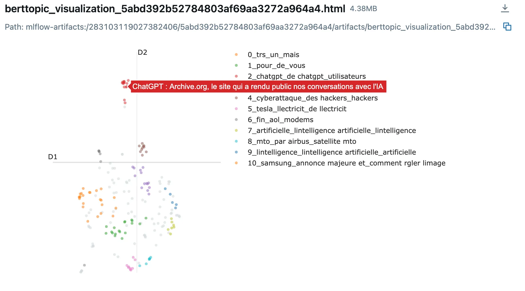
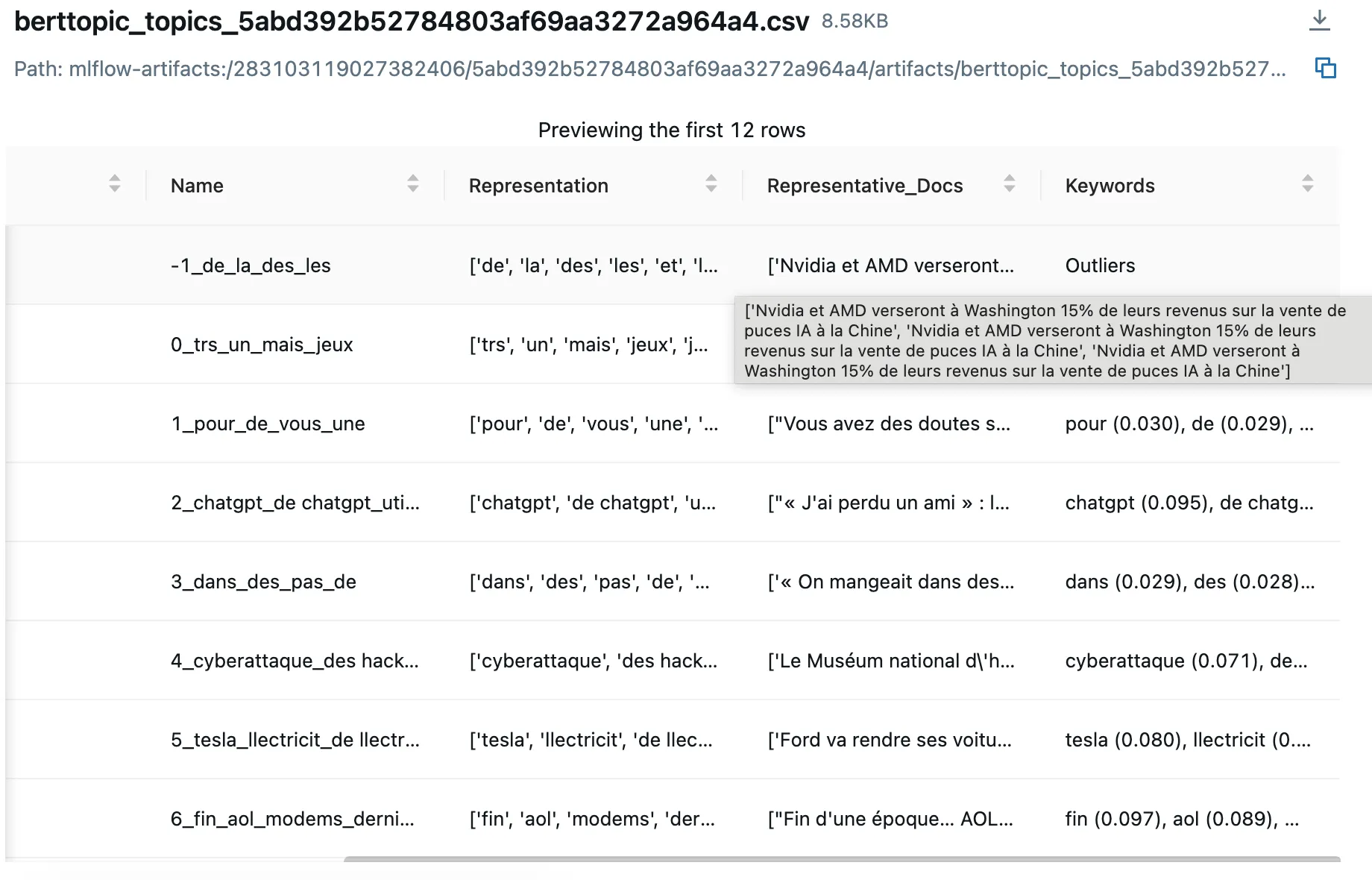
- Representative Documents: Review actual text samples from each cluster to assess quality
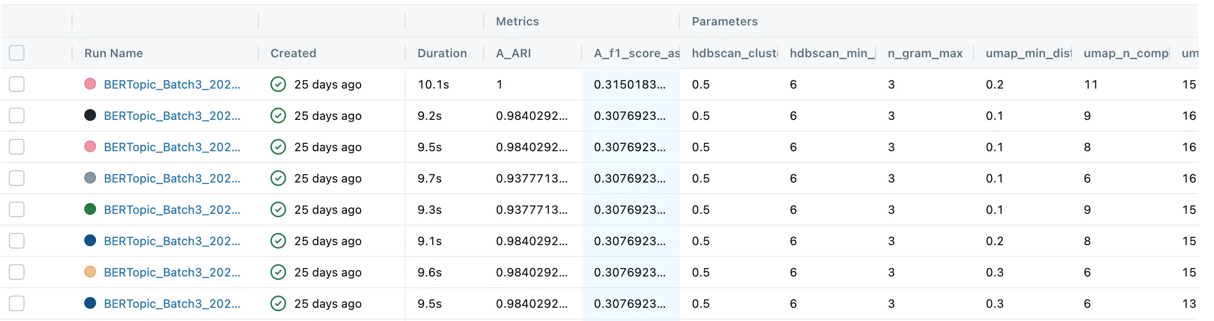
- Metric Comparisons: Sort and filter experiments by any logged metric
The MLflow UI (accessible at http://localhost:12001 in the repo) becomes your command center for understanding which combinations work best.
Key Insights and Conclusions
After building and using this system extensively, here are my main takeaways:
Speed Through Smart Optimization
By pre-computing embeddings and parallelizing experiments, I can test hundreds of parameter combinations in just tens of minutes. The embedding cache and ProcessPoolExecutor combination is the secret sauce here.
Discovering Unexpected Configurations
The system revealed parameter combinations I never would have tried manually. For instance, I now have a production configuration running with:
{
  "umap": {
    "n_neighbors": 25,
    "n_components": 15
  }
}
No tutorial or LLM ever suggested parameters this high, but for my specific dataset, they work brilliantly.
The Human Element Remains Critical
While I’m automating the downstream pipeline (dataset generation, automated experimentation launches), I haven’t automated the final configuration export - and I’m not sure it would be desirable. Often, the top-performing combinations are very close in metrics, and I need to:
- Analyze the results carefully
- Test them in production
- Make a final decision based on real-world performance
The best configuration on paper isn’t always the best in practice. Sometimes a slightly lower-scoring configuration produces more interpretable or stable topics in production.
Looking Forward
This system has transformed how I approach NLP clustering. Instead of guessing parameters based on vague intuition or generic recommendations, I can systematically explore the parameter space and find what actually works for my data.
The combination of BERTopic’s flexibility, MLflow’s tracking capabilities, and Python’s parallel processing creates a powerful experimentation platform. Whether you’re clustering news headlines, customer feedback, or any other text corpus, this approach can help you find the optimal configuration for your specific use case.
Feel free to explore the source code and adapt it for your own projects.